How to measure Lead Quality using Google Spreadsheet and Cohort Analysis.
What is the number one complaint which comes from the Sales team ?
In my brief experience managing a Sales team, the key complaint which typically comes up is - “Leads are not good as they were before”. Week after week this used to come up and it still comes up. Now quantifying that was not easy unless I ran a cohort analysis.
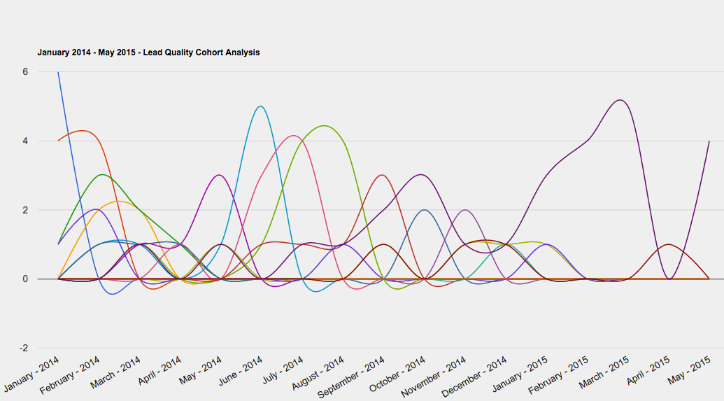
Here is the output of the cohort analysis I ran using Google Spreadsheets.

There are 5 broad steps to measuring lead quality using cohort analysis :
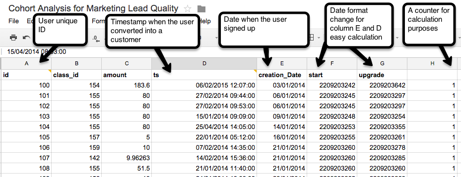
1.Get the data around when the user signed up and registered
This should include all users who registered / signed up using your “Free Trial” or “30 Day Trial”. This ideally would contain the unique identifier for the user and the timestamp when they signed up on.
Here is a link to the sample google spreadsheet for user registration. The second sheet (User Signup Data) contains the user information. The key information to start off is in column A, D and E.
2.Add additional data around when the user converted to a customer

This is the timestamp around when the user converted into a customer (a paid user). This is essentially column D (ts) in the same sheet
3.The real cohort
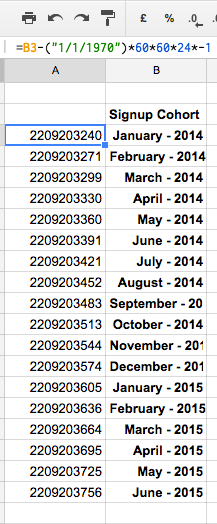
The third sheet will contain the months for which you need to do the analysis both in the column and the row. We also will convert the date into the UNIX timestamp format.

This same thing is also applied across for the months at the top.
After you get this basic matrix, then the real magic is using the “SUMIF” within each of the cells to get the answer to “Get me the count of users who signed up this month and also became a customer”. The formula looks like this in the google spreadhseet.
=SUMIFS('Users Signup Data'!$H$2:$H$118,'Users Signup Data'!$F$2:$F$118,">"&$A$3,
'Users Signup Data'!$F$2:$F$118,"<"&$A$4,'Users Signup Data'!$G$2:$G$118,">"&C1,
'Users Signup Data'!$G$2:$G$118,"<"&D1)
You can look at the individual columns for each of the month the google spreadsheet.
We also found out the total new revenue we got based on the conversion which is towards the end of the spreadsheet.
=SUMIFS('Users Signup Data'!$C$2:$C$118,
'Users Signup Data'!$F$2:$F$118,">"&A3,'Users Signup Data'!$F$2:$F$118,"<"&A4)
What are the key things we learned ?
These are the lessons learned :
- That we could find out lead quality by revenue generated over a period of time.
- In the sample sheet lead quality has actually decreased.
- You don’t need complicated models to measure lead quality (as you see a simple Google spreadsheet and formulas will help you get the results you need)
